camtraptor 1.0.0

We just released a new major version (1.0.0) of our R package camtraptor.

With camtraptor you can explore and visualize Camera Trap Data Packages (Camtrap DP). It offers a step-by-step workflow to read Camtrap DP files, filter data of interest, summarize information (e.g. number of observed species) and visualize this per deployment on an interactive map. You can also use it to transform data for analysis in camtrapR.

This major release updates the internal data model of camtraptor to Camtrap DP 1.0, drops support for Camtrap DP 0.1.6 and facilitates a step-by-step exploration workflow with new functions.

What has changed?

camtraptor now offers a step-by-step workflow to explore and visualize data:

1. Read Camtrap DP files with read_camtrapdp() (reexported from camtrapdp::read_camtrapdp()). This function supports Camtrap DP 1.0 or higher.
2. Filter the data with filter_deployments(), filter_media() and filter_observations() (also reexported from {camtrapdp}). These functions replace the predicate functions (which only worked on deployments) and filter arguments in get_ functions.
3. Summarize deployments and observations with summarize_deployments() and summarize_observations(). These calculate features (e.g. effort_duration or n_events) grouped by fields (e.g. deploymentID, latitude and longitude) and temporal levels (e.g. "month") of your choice.
4. Visualize those summary tables using map_summary(), which creates a Leaflet map for the desired feature. This function replaces map_dep().

Here’s an example where you read files, filter on coordinates and adult animals, calculate observation-level summaries, and create a map showing the number of individuals:

library(camtraptor)
file <- "https://raw.githubusercontent.com/tdwg/camtrap-dp/1.0/example/datapackage.json"
x <- read_camtrapdp(file)
x %>%
  filter_deployments(latitude > 51.0, longitude > 5.0) %>%
  filter_observations(lifeStage == "adult") %>%
  summarize_observations() %>%
  map_summary(feature = "sum_count")

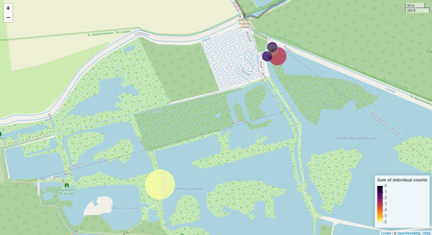
Note how you can stop and explore (all) the summary results returned by summarize_observations() before selecting one ("sum_count") to visualize with map_summary():

# A tibble: 4 × 10
# Groups:   deploymentID, latitude, longitude, scientificName [4]
  deploymentID latitude longitude scientificName     n_scientificName n_events n_observations sum_count rai_observations rai_count
  <chr>           <dbl>     <dbl> <chr>                         <int>    <int>          <int>     <int>            <dbl>     <dbl>
1 29b7d356         51.2      5.66 Anas platyrhynchos                1        3              3         6             30.1      60.3
2 577b543a         51.2      5.66 Martes foina                      1        1              1         1             11.0      11.0
3 577b543a         51.2      5.66 Mustela putorius                  1        3              3         3             32.9      32.9
4 577b543a         51.2      5.66 Vulpes vulpes                     1        1              1         1             11.0      11.0

More details about the new workflow can be found in the vignette Workfow. Do you want more info about the visualization aspect? Give a look to the vignette Visualize deployment features. For an overview of all the changes, see the CHANGELOG.

How to install camtraptor?

Want to use camtraptor in your work? The package is available on GitHub and can be installed with:

# install.packages("pak")
pak::pak("inbo/camtraptor")

For more information, see the package documentation. Found a bug? Please report an issue.